MTBF Paradox: Case Study

Guest Post by Msc Teofilo Cortizo

The MTBF calculation is widely used to evaluate the reliability of parts and equipment, in the industry is usually defined as one of the key performance indicators. This short article is intended to demonstrate in practice how we can fool ourselves by evaluating this indicator in isolation.

We get real data from two failure modes of a conical crusher drive system: failure of the electric motor and failure of the grid spring coupling. With the use of reliability software it was possible to estimate in two parametric Weibull modeling 2 parameters, that is, the gamma parameter (γ) = 0:

Electric Motor Failure

β = 0,46

η = 3491

Grid Spring Coupling Failure:

β =0,24

η = 857

By the characteristics of the value of the two parameters, we conclude that the coupling failure has a higher probability of occurring at the beginning of its life. Based on this modeling it is possible to calculate the MTBF of each failure mode:

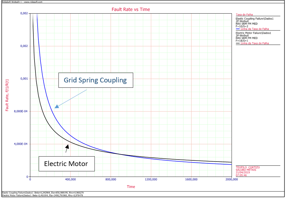
We note that the calculated MTBF for coupling failure is almost three times greater than that of the electric motor. The analysis of this indicator alone would lead us to believe that the fault in the electric motor is more critical than that of the grid spring coupling. However, we observe from the modeling analyzes that there is a higher probability of failure at the beginning of the life of the coupling. How can we explain this phenomenon? Let us analyze the graphs of failure rates over time of the two failure modes studied:

See that there is a higher failure rate over time for grid spring coupling and after 800 hours of life, the curve is reversed pointing the electric motor to be the most critical. Let’s look at the probabilities of failure over time.

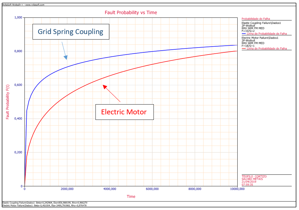
The probability of failures of the grid spring coupling is greater than that of the electric motor throughout the year. By simulating the events in block diagram using the Monte Carlo method we confirm this interpretation.

With fault data, you can also get the repair data. To simplify, we have adopted two exponential models with their average repair times:

With fault and repair curves we performed 5000 simulations over a year of life.

We now compare the criticality results of failure modes by both number of events and unavailable time:

The big question is: if the modeling parameters, probability curves and reliability simulation pointed to failure in the elastic coupling being more critical than the motor failure, why is the MTBF higher?

Two considerations must be made, the MTBF parameter is easier to compare when failure modes follow a random or exponential curve modeling. Thus, there are constant failure rates over time and the MTBF can be used as an indicator that represents its reliability. Second point is that the calculation of the MTBF by the reliability systems takes into account an infinite life time. Until the probability area of f (t) becomes 100% over a long period, remember that the PDF of these equipments presents as an exponential function and its characteristic is to present an asymptotic curve with the horizontal axis. In summary, in the exponential function the curve meets the horizontal and vertical axis in infinite time.

We can prove this thesis if we increase much more the simulation time.

As we can prove, after 20 years of life, engine failure becomes more critical than that of the grid spring coupling. Lets check the fault probability graph in 50000 hours:

Next to 20 thousand hours of working, the probability behavior changed. The electric motor show up as a most critical.

CONCLUSIONS

We must be careful when using the MTBF as a solitary indicator of reliability. We have to be aware of the behavior of the equipment (if it would suit an exponential) and how much time we are evaluating the criticality of the assets. The ideal is to use several indicators for comparison and whenever possible perform reliability models of the main assets to have assertiveness of their behavior over time.