MTBF: What is it Good For?

Guest post by Andrew Rowland, CRE, ReliaQual Associates, LLC

I.  INTRODUCTION

The mean time between failure (MTBF) is arguably the most prolific metric in the field of reliability engineering. The MTBF is used as a metric throughout a product’s life-cycle; from requirements, to validation, to operational assessment. Unfortunately, MTBF alone doesn’t tell us too much.

It’s not that MTBF is a bad metric. The problem is MTBF is an incomplete metric and, as an incomplete metric, it doesn’t lend itself to risk-informed decision making. The real problem is not with the MTBF, it is with the implicit assumption that failure times are exponentially distributed.

In the following discussion, we will look at two examples where the MTBF alone could lead us to bad decision making.

II.  EXAMPLES

To illustrate how relying on the MTBF can be misleading, let’s look at two examples. In these examples we will assume the failure times are Weibull distributed. The Weibull distribution is popular in reliability engineering and the exponential is a special case of the Weibull. From the literature we know the probability density function and survival (or reliability) function of the Weibull can be expressed as follows:

$latex \displaystyle&s=4 f\left( t \right)=\left( \frac{\beta }{\eta } \right){{\left( \frac{t}{\eta } \right)}^{\beta -1}}{{e}^{-{{\left( \frac{t}{\eta } \right)}^{\beta }}}}$

$latex \displaystyle&s=4 S\left( t \right)={{e}^{-{{\left( \frac{t}{\eta } \right)}^{\beta }}}}$

We also recall that the mean of a Weibull distributed variable can be estimated as:

$latex \displaystyle&s=4 MTBF=\eta \Gamma \left( 1+\frac{1}{\beta } \right)$

In the functions above, η is referred to as the scale parameter and β the shape parameter.

A.  Example 1

Consider  three  items; Item A, Item B, and Item C.  Perhaps the goal is to select one of these items for our design and the requirement   is to  have  a  90 hour  MTBF   or  greater.  All  three  items  have  an  MTBF   of  100 hours. So, from a reliability perspective, which is the Item to choose?

Under the implicit assumption that failure times are exponentially distributed, we might conclude that any of the three is acceptable, reliability-wise. All three satisfy the 90 hours MTBF requirement. However, let’s look a little deeper into the 100 hour MTBF and see if we still agree that any of the three is acceptable.

Let’s take a look at the reliability over time of each Item. Figure 1 shows the reliability function over 500 hours for each of these Items. Clearly, the reliability of these Items  is not the same.  Given that each Item has an MTBF of    hours, what is the reliability at 100 hours? Table I summarizes the 100  hour reliability for each Item. Once again, we can see a large difference between the three Items.

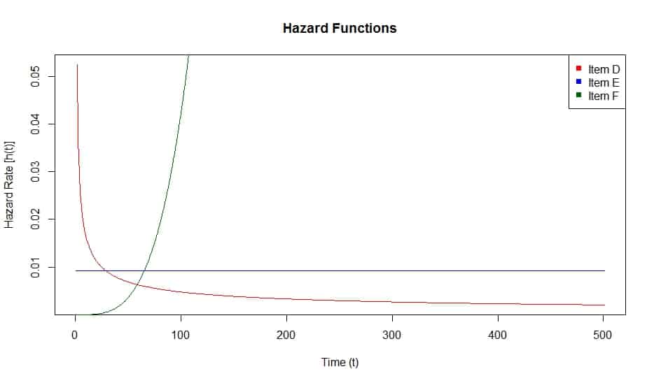
Another way to compare these three Items is via the hazard, or failure, rate. Figure 2 shows the hazard function for each Item. The “bathtub” curve is a plot of hazard rate versus time. Thus, Figure 2 shows the “bathtub” curve for each Item. Clearly the hazard rate behavior is very different for these Items.

Fig. 1.   Reliability Functions for Item A, Item B, and Item C

TABLE I
RELIABILITY AT 100 HOURS FOR ITEM A, ITEM B, AND ITEM C

Item	R(100)
Item A	0.109 (10.9%)
Item B	0.367 (36.7%)
Item C	0.521 (52.1%)

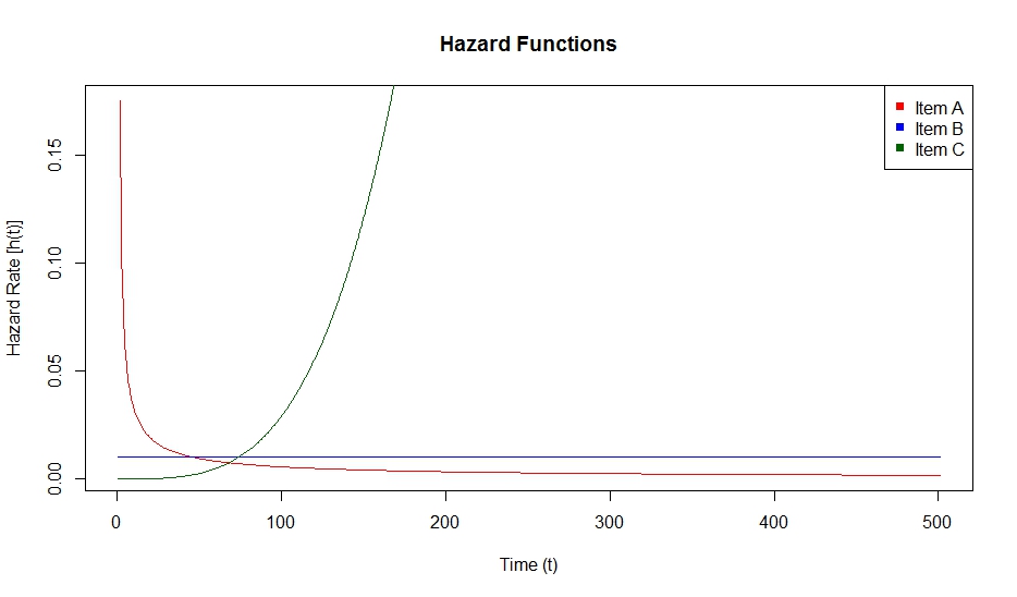
Fig. 2.   Hazard Functions for Item A, Item B, and Item C

B.  Example 2

Consider another situation where we have three items; Item D, Item E, and Item F. Presume for a moment that we have all of the data used to derive the MTBF statistic for each Item. The first thing we might do is graphically explore the data. Figure 3 shows a set of plots commonly used in graphical analysis of survival data for Item D. Let’s look at the histogram in the upper left corner. We see the distribution is heavy-tailed indicating failure times are not exponentially distributed.

Compare the histogram in Figure 3 to that in Figure 4 for Item E and Figure 5 for Item F. Clearly the distribution of failures times differs amongst these three items. Yet all three items have the same MTBF. Perhaps we need to look a bit closer at the data!

Now that we’ve graphically analyzed the data and concluded we may be looking at different populations, we decide to fit the data to a distribution and estimate the parameters.

Our goal, then, is to estimate the value of β and η for each Item. We use the fitdist function from the R [1] package fitdistrplus [2]  which uses maximum likelihood to estimate  the parameters. The results for these three populations are summarized in Table II. We can see from these results that the populations are not the same, although all three Items satisfy our 90 hours MTBF requirement.

Now that we’re confident we’re dealing with three different populations all with the same MTBF, what is the implication of selecting one Item over another? Since we fit the data to a Weibull distribution, we know the shape parameter (β) determines the region of the “bathtub” curve. With a β < 1, we are in the early life region, a β = 1 puts us in the useful life region, and a β  > 1 indicates wearout.  In other words, Item  D is dominated by early-life failure mechanisms, Item E is by useful life failure mechanisms, and Item F by wearout.

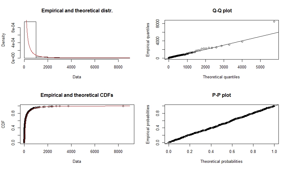
Fig. 3.   Item D: Graphical Analysis of Survival Data

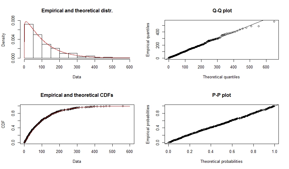
Fig. 4.   Item E: Graphical Analysis of Survival Data

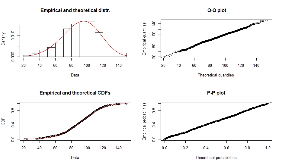
Fig. 5.   Item F: Graphical Analysis of Survival Data

As we  did with the first  example, let’s look at the  reliability function  for  these  three  Items. Figure 6 shows the reliability functions. Similar to the first example, we see the reliability functions are not the same as we would expect from our assessment of Figure 3, Figure 4, and Figure 5.

Fig. 6. Reliability Functions for Item D, Item E, and Item F

Let’s assume we are interested in the reliability at 50 hours. The reliability at 50 hours for the three Items can be found in Table III. We see a dramatic difference in the reliabilities and, interestingly, the Item with the highest 50 hour reliability is the Item with the lowest MTBF.

We can also look at plots of the hazard function for these three Items. These hazard functions are plotted in Figure 7 over 500 hours. We see different hazard rate behaviors as we expected from our assessment of the β values we estimated earlier. TABLE II

ESTIMATED PARAMETERS FOR ITEM D, ITEM E, AND ITEM F

Item	R(100)	Beta	MTBF
Item D	101.42	0.478	220.7
Item E	107.73	1.000	107.7
Item F	100.84	4.524	92.0

TABLE III

RELIABILITY AT 50 HOURS FOR ITEM D, ITEM E, AND ITEM F

Item	R(50)
Item D	0.490 (49.0%)
Item E	0.645 (64.5%)
Item F	0.959 (95.9%)

Fig. 7. Hazard Functions for Item D, Item E, and Item F

III.   CONCLUSION

Hopefully we’ve come to understand that stating an MTBF value with no other information doesn’t really tell us much about the reliability of an Item. Neither does it tell us if the Item truly satisfies our reliability needs. We saw in one example three Items with the same MTBF, but most definitely with different reliability behavior.

In the second example, we looked at three Items with different MTBF. Once again, we saw the reliability behavior of these Items were different. In this example we saw the Item with the largest MTBF having a 50 hour reliability almost half that of the Item with the lowest MTBF.

Without an understanding of the reliability characteristics that is more complete than simply MTBF are we making good, risk-informed decisions? Selecting Item A or Item D, we can expect to see high rates of failure during validation, reliability growth testing, or, worse yet, early in customer ownership. If we warrant our product, we can expect large warranty costs associated with Item A or Item D. Given the competing requirements we need to satisfy, we may need to select Item A orItem D. If we only know the MTBF will we put the necessary barriers in place, such as screening, to minimize the risk?

At the other end of the “bathtub” curve, if we select Item C or Item F, our validation or reliability growth testing may not test far enough into wearout to surface failures. Will we develop a preventive maintenance program for these Items to minimize the risk?

MTBF is ingrained in the reliability community as well as throughout most companies. It is unlikely that we will ever see the end of MTBF. Ultimately it comes down to us, as reliability engineers, to understand the limitations of MTBF and educate those around us to it’s shortcomings. If the reliability community gets in lock-step, we can be the tugboats that change theship’s heading.

REFERENCES

[1]  R Development Core Team, R: A Language and Environment for Statistical Computing.            Vienna, Austria: R Foundation for Statistical Computing, 2009.

[2]  Marie Laure Delignette-Muller and Regis Pouillot and Jean-Baptiste Denis and Christophe Dutang, fitdistrplus: help to fit of a parametric distribution to censored or non-censored data. 2013

Andrew Rowland is a Reliability Consultant. He previously worked as a Reliability and Safety Engineer in the aerospace, defense, and civil nuclear industries. Mr. Rowland received a BSEE in 1999 and a MS in Statistics in 2006. He is an American Society for Quality Certified Reliability Engineer, a member of the IEEE Reliability Society, and the American Statistical Association. He may be contacted by email at andrew.rowland@reliaqual.com.

For a pdf copy download from slideshare