Introduction
How is a manufacturing process determined to be capable of producing parts that meet engineering requirements? Some, like the finish of a gear tooth are critical, while the roughness of a non-contact surface isn’t critical. The critical characteristics need to be identified and checked to determine if the process is capable.
This article defines the analysis concepts and indices.
Prototypes and Series Production
Process capability assessments (PCA) start during the product development process and continue into series production. Prototype parts are created by a variety of methods, ranging from hand-crafted parts to short term manufacturing in a production intent process under factory conditions. The methods that are closest to series production are the most realistic.
The Data
The data collected on critical characteristics show a central value and variation. It is relatively easy during development and during serial production to adjust the central value while variation is hard to control. A normal distribution provides a good model for many measurements.
For prototype part data the sample mean, $-\bar{X}-$, and standard deviation, s, are calculated, using equations 1 and 2.
$$\bar{X}=\sum_{i=1}^{i=N}X_i$$
(1)
$$s^2=\sum_{i=1}^{i=N}\frac{(X_i-\bar{X})^2}{N-1}$$
(2)
For serial production, SPC can be used to estimate the process mean and standard deviation. If $-\bar{X}-$ and R charts are used, then the overall process average, $-\bar{\bar{X}}-$, and the standard deviation, s, are calculated using equations 3 and 4.
$$\bar{\bar{X}}=\sum_{j=1}^{j=N}{\bar{X}_j}$$
(3)
$$s=\frac{\bar{R}}{d_2}$$
(4)
The average and standard deviation are used to estimate the normal distribution parameters, $-\mu-$ and $-\sigma-$, ignoring sample variation. The 3$-\sigma-$ limits of the distribution are calculated using equation 5.
$$\mu\pm3\sigma$$
(5)
Note the distribution 3$-\sigma-$ limits have a range of 6$-\sigma-$.
A Centered Process
When there is a two-sided engineering specification, the middle of the tolerance range is the usually the process target. In some specifications, there may be a non-centered target, but that is not discussed in this article. A normal distribution with a centered process is shown, figure 1.
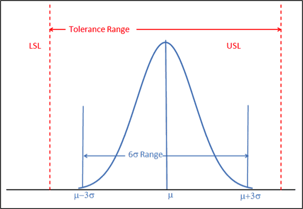
Figure 1
The ratio of the tolerance range to the 6s range is calculated in equation 6.
$$\frac{USL-LSL}{6\sigma}$$
(6)
If prototype parts were used to estimate $-\mu-$ and $-\sigma-$,
then the ratio in equation 6 is called the Process Performance, Pp. Alternatively, if SPC samples from a series process were used, then the ratio is the Process Capability, Cp.
There are three cases for centered normal processes with a 2 sided-tolerance specification, figure 2.
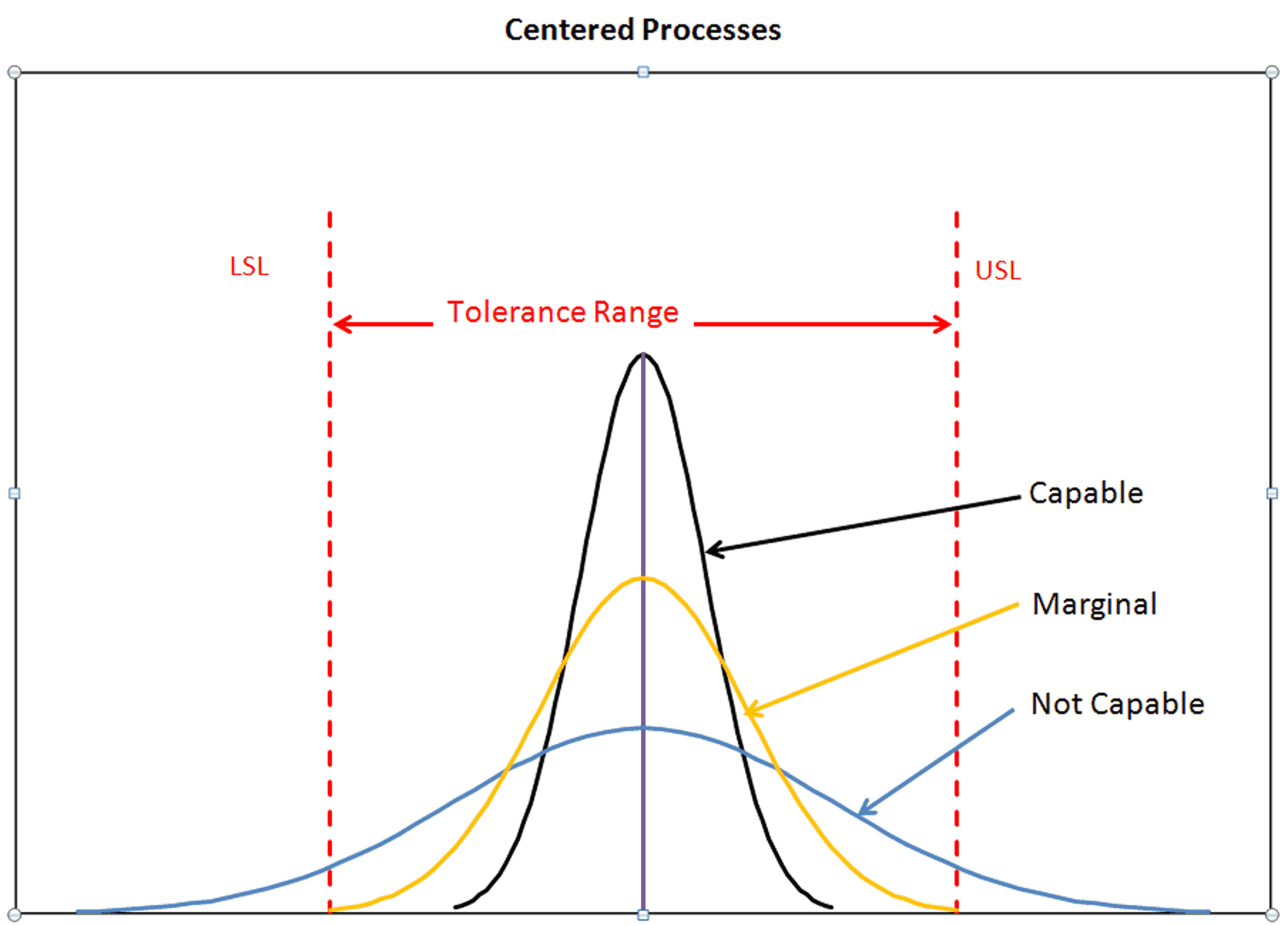
Figure 2
The greater the variation, the harder it is for a process to be capable. A capable process shown in black is within the tolerance limits and has a Cp (or Pp) = 1.67! A process that is not capable is shown in blue, has a Cp = 0.67. The distribution tails cross the specification limits, allowing the production of non-conforming parts. The marginal process shown in yellow has 3$-\sigma-$ distribution limits that just touch the tolerance limits. The marginal process Cp = 1. In marginal process, any change in the process average causes a tail of the distribution to cross the tolerance limit, allowing for non-conforming parts to be produced.
Some corporations target $-P_p\geq{1.67}-$ and $-C_p\geq{1.33}-$! Six Sigma practitioners target $-C_p\geq{2}-$, for a process under statistical control.
Non-centered Processes
The best performance comes from a centered process. A non-centered process produces more defectives than a centered process. Consider three distributions with the same spread, but different centers in figure 3.
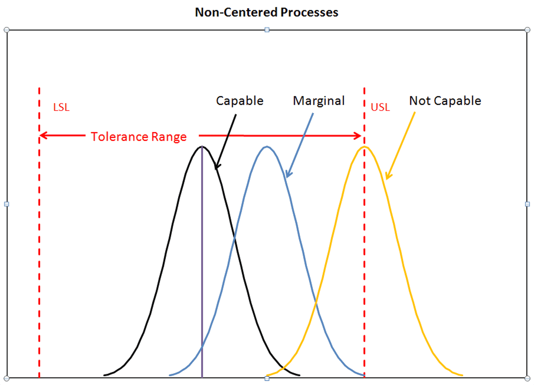
Figure 3
Here the process represented by the black distribution is capable; the blue distribution, marginal; and the yellow distribution, not capable. The process described by the yellow distribution produces about 50% non-conforming for the measured characteristic.
The gap between the closest tolerance limit and the center of the distribution is divided by 3$-\sigma-$ and captures the centering effect, figure 4. and equation 7.
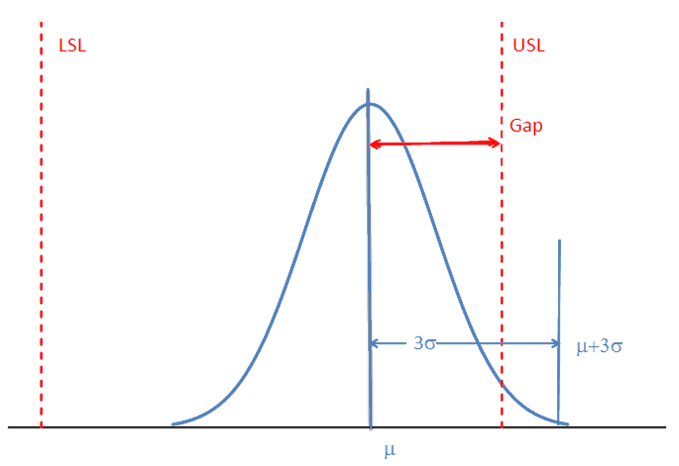
Figure 4
$$\frac{min(USL-\mu,\mu-LSL)}{3\sigma}$$
(7)
If prototype parts were used to estimate μ and σ, then the index, calculated in equation 4, is Ppk. If the data came from series production, then the index is Cpk.
If the 6$-\sigma-$ range is much smaller than the tolerance range, then the process center can shift but remain capable. If the 6$-\sigma-$ range is equal to or larger than the tolerance limits, then the process is not capable and needs to be improved. Identifying and controlling factors that contribute to process variation can accomplish this, but this is a topic for another article.
For a capable process, the indices Pp, Ppk, Cp, and Cpk, must to be greater than 1. For pro-type parts, some organizations want both Pp and Ppk, to be greater than 1.67! Because series production should include all sources of variation, some organizations want Cp and Cpk to be greater than 1.33!
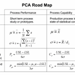
PCA Road Map
These concepts, for two sided tolerances can be captured in a PCA Road Map in table 1.
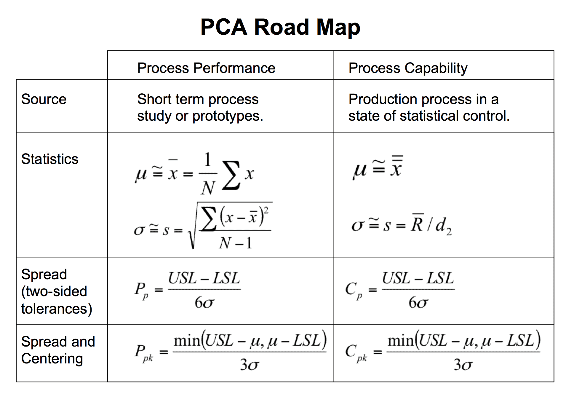
Table 1
Note the different statistical calculations in the second row. Both are recognized methods of estimating the mean, μ, and standard deviation, σ. In the second column, the source is a small sample of prototypes. In the third column, the source is production SPC.
One-sided Engineering Specifications
Some engineering tolerance are don’t have both an upper and lower specification limit. Frequently, physical constraints do not permit negative values. Some examples are surface roughness, wheel or tire radial run-out, the electrical resistance of electronic switches. In these situations, only an upper specification limit is necessary.
In this situation, the tolerance range is unbounded on the undefined limit. It is not possible to calculate a Pp or Cp index. However, the Ppk and Cpk indices can be calculated using equation 7 with the defined specification limit.
Conclusions
A process capability analysis can determine if a process is capable of producing parts that conform to engineering specifications. While prototype parts can provide preliminary process performance information, the final process capability assessment must be based on series production.
The final capability index is highly dependent on the process being centered between tolerance limits and variation needs to be smaller than the tolerance range.
Next
The next article discusses how to estimate Percent Defectives.
Note
If you want to engage me as a consultant or trainer on this or other topics, please contact me. I have worked in Quality, Reliability, Applied Statistics, and Data Analytics over 30 years in design engineering and manufacturing. In the university, I taught at the graduate level. Also, I provide Minitab seminars to corporate clients, write articles, and have presented and written papers at SAE, ISSAT, and ASQ. I want to assist you.
Dennis Craggs, Consultant
Quality, Reliability and Analytics Services
810-964-1529
dlcraggs@me.com
Very nice article…. Thanks a lot…
Would be interesting to know some history how this limit of 1.67 and 1.33 arrived at for the Process Performance and Process Capability…!!
I need to do some research on the history, but different companies set different targets. For example, the Six Sigma people have a rational for Cpk >= 2.0 that allows for some the process center to wander over a +/- 1 sigma range.
Other organizations don’t set a target, but their operating policy is to continually reduce variation. Their belief is that reducing variation will not only reduce defects but improve the function.
Examples:
1) An American auto company wanted their European group to use a US manufactured transmission. The European group wanted to use a high quality European source. The US manufactured product had Cpk’s of approximately 1. However, the European competitor had a Cpk’s of approximately 13. The decision was to stay with the European source.
2) A blind study of a Japanese transmission performance with the US transmission showed better customer ratings for the Japanese product. A study was made to compare the products. The designs were the same, but the variation in the Japanese transmission could not be measured. The US manufacturer needed to purchase an improved measurement system to even measure variation in the Japanese transmission components. The Japanese designers positioned their processes within the US specifications to minimize noise and harshness, improving performance.
Look at Taguchi’s Loss Function idea.
Missing right bracket equation (7).
Thanks for finding the typo.