
The Situation
You have a process that is not capable because sample measurements or SPC data indicate that some characteristics have too much variability. The calculated Cpk’s are too small. What do you do?
Assuming the data is correct, a course of action is to review the assumption is that the measurements are normally distributed. For most situations, this is a reasonable assumption, but other statistical distributions may provide a better description of the data variation.
Central Limit Theorem
In Wikipedia, you will find the following definition
In probability theory, the central limit theorem (CLT) establishes that, in most situations, when independent random variables are added, their properly normalized sum tends toward a normal distribution (informally a “bell curve”) even if the original variables themselves are not normally distributed. The theorem is a key concept in probability theory because it implies that probabilistic and statistical methods that work for normal distributions can be applicable to many problems involving other types of distributions.
Components may be connected and the interfaced dimensions stack-up to yield an assembly dimension. When the dimensions are additive, the central limit theorem applies. In other situations, the stack-up relations may be non-linear. If the tolerance ranges are tight, the stack-up may be approximately linear. The normal distribution works well where the stack-up of component dimensions is approximately linear.
The normal distribution is then used to describe the bulk of the data. Sometimes outliers from the normal distribution are shown in the upper and lower tails. The normal distribution equation predicts a finite probability for extremely low or high tail values. Physical limits in the real world may prohibit extreme values. Some examples of physically constrained values are negative electrical resistance or infinite weight for a part.
Other Distributions
Since the physics limit the potential values of a parameter, what distribution should be considered? Weibull and Lognormal distributions should be considered where physical limits constrain to be greater than 0. Weibull is very good at describing life data and the Lognormal is good at describing parameter data.
Case Study
A supplier was required to calculate the process capability for electrical resistance of an electrical switch when the device was conducting current.
The engineers need low electrical resistance to avoid heating a module containing the electrical switch so the switch design is biased to yield low resistance values.
The customer’s specification for the resistance was 15±15 milliohm which yielded a Lower Specification Limit (LSL) of 0 milliohm and an Upper Specification Limit (USL) of 30 milliohm. From SPC data, the electrical resistance averaged 2.77 milliohm and had a standard deviation of 2.01 milliohm. So the Cpk=0.52, much less than the desired Cpk≥1.33!
Using the mean and standard deviation, the lower 3s limit was calculated to be -3.23 milliohm. Also, the probability of resistance values being less than 0 is 8.3%. This is not physically possible. This provides clues on how to improve the analysis:
- LSL is not needed since the resistance is constrained to be greater than 0 by physical processes. Only the USL needed to be considered in the calculation of Cpk.
- The normal distribution is inadequate to describe the data distribution. The probability of negative resistance values is too high. An alternative distribution should be used.
In this situation, the Cpk calculation should use only the USL. If the data followed a normal distribution, then
$$C_{pk}=\frac{30-2.77}{3*2.01}=4.516$$
This would be acceptable, except for the fact that the data is not normally distributed.
To identify the best distribution, the 50 resistance values were plotted using the Weibull, Lognormal, Exponential, and Normal probability plots, figure 1.
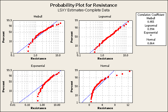
Figure 1
The box in the upper right of Figure 1 shows the lognormal distribution provides the best fit to the data with a correlation of 99.1%. The closer that the data points follow the blue line for each distribution plot, the better the fit. The worst distribution to use would be the exponential. It shows a lot of deviation from the blue distribution line. Similarly, the normal distribution is not a good choice. The lognormal distribution provides the best fit to the data distribution, but some small deviation occurs on the distribution tails. The Weibull is the 2nd best distribution to consider. For the remainder of this case example, only the lognormal will be discussed.
Assuming that the resistance values, x, are log normally distributed and the log of the resistance values are normally distributed. The calculating procedure should be:
- Calculate the average of the log of the resistance values: $-\bar{y}=\frac{1}{N}\sum{ln(x_i)}=0.7-$
- Calculate the standard deviation of the log of the resistance values: $-s=\sqrt{\frac{\sum{ln(x_i)-\bar{y}}}{N-1}}=0.7-$
- Calculate the log of the USL: $-ln(USL)=ln(30)=3.40-$
- Calculate the Cpk: $-C_{pk}=\frac{ln(USL)-\bar{y}}{3s}=\frac{ln(30)-0.7}{3(0.7)}=3.07-$
A Cpk=3.07 is reasonable in this case as it ignores the LSL, considers the USL, the lognormal distribution of the data, and the physical principles that mandate positive values of electrical resistance.
Conclusions
A critical characteristic needs to be analyzed to assure the data is normally distributed, before calculating process capability. If an alternative distribution is used, then a transformation of the data and specification limits are required prior to calculating the Ppk or Cpk.
The basic definition of Ppk and Cpk assume there are a lower and an upper specification limit. Sometimes, physical principles restrict the values that are possible, so one of the specification limits is not necessary. In that situation, the Ppk and Cpk calculations are simplified.
Do you have manufacturing and design problems? I worked for 30 years solving design engineering and manufacturing problems by applying Quality, Reliability, Applied Statistics, and Data Analytics. If you want to engage me on this or other topics, please contact me. I taught undergraduate statistics; reliability and robust design at the graduate level. I provide Minitab seminars to corporate clients, write articles, and have presented and written papers at SAE, ISSAT, and ASQ. When software tools are not available to support the analysis process, I write custom software for the job.
Dennis Craggs, Consultant
810-964-1529
dlcraggs@me.com
Sir,
What are Pkp and Cpk?
please explain the abbreviations/notations.
The first article in the process capability series defined and discussed the capability indices Ppk and Cpk. Both Ppk and Cpk are ratios. In the numerator is the measured difference between the process center and the closest tolerance limit. In the denominator is 3$-\sigma-$. If $-\mu-$ and $-\sigma-$ are calculated from a small short term sample, it ignores some factors of variability and is called Ppk. If$-\mu-$ and $-\sigma-$ come from long term SPC chart, shows the process is stable and in statistical control, then it is called a Cpk. These were defined in the first article on the topic. Try this link to the first article.
https://lucas-accendo-site-speed.sprod01.rmkr.net/process-capability-analysis-i/
Thank you for this information rich and clearly written article on calculating Cpk.
I am struggling with the idea of using “Cpk” as a capability statistic when the data is non-normal and there is a unilateral tolerance. I am currently doing a study with an actual process that measures flatness with a specification of ‘less than .015″ and I have tons of data over long periods of time to work with.
I am trying different ways of calculating Cpk or a Cpk-like number and then correlating it with actual rejection rates to determine if thee calculated value has any predictive value such as a proper Cpk (as in bilaterally toleranced and normally distributed).
I was a joy to discover your clearly written article. It addressed the questions I have been struggling with and gave me hope that you might be able to help me wrap my head around this. I have a very good conceptual grasp of Cpk and feel I relate it well to others. However, this grasp is deeply compromised when moving away from the standard assumptions.
One question I have is this:
The entire spread of the distribution of data needs to fall below the ULS. Therefore, wouldn’t we have to divide the spread by 6 sigma (both sides of the transformed curve) or at least add the mean to the 3 sigma to account for the part of the curve to the left of the ‘new normal’?
Hi Fred, I apologize for my very late reply. You have data, and probably a specification, for flatness. If your measurement system provides a single number for each sample, then this would represent part-to-part variation. How is this defined? Perhaps the max – min on a part.So does the data approximately fit a known distribution? In my experience, flatness does not conform to a normal, for a start you could try Weibull, lognormal, chi-square, or perhaps extreme value. The requirement should be a one-sided upper bound specification because for flatness, smaller is better. Generally, one gets into trouble when the flatness measurement is large.
On a single part, the flatness would represent within-part variation. How could this be measured, perhaps as a root mean square. Would it be normal? Probably not, but try different distributions.