Introduction
In prior articles on process capability, sample statistics and SPC statistics were assumed to be population parameters and ignored sampling variability. This article reviews the analytic methods that can be used to develop confidence bounds on the process capability indices.
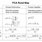
$-P_p-$ Index
The Pp index calculation requires an estimate of the parameter σ. The index is calculated as:
$$P_p=\frac{USL-LSL}{6\sigma}$$
(1)
The parameter σ is estimated from the sample standard deviation s, ignoring sampling variability. However, the sample variance s2 follows a Chi-square distribution with n-1 degrees of freedom. The $-\chi^2-$ statistic is:
$$\chi^2=\frac{(n-1)s^2}{\sigma^2}$$
(2)
Combining equations 1 and 2 yield:
$$P_p=\frac{USL-LSL}{6s}\sqrt{\frac{\chi^2}{(n-1)}}$$
(3)
Equation 3 is similar to equation 1 with an additional factor $-\sqrt{\chi^2/(n-1)}-$that corrects for sample variation.
Equation 3 is used to calculate Pp index confidence limits by using values of $-\chi^2-$ that correspond to percentiles on the Chi-square distribution with n-1 degrees of freedom.
Example
A part characteristic has the specification 10±0.2 (LSL = 9.8 and USL= 10.2). A critical characteristic was measured for 30 sample parts and a sample standard deviation of 0.065 was calculated. The 0.065 was used for population $-\sigma-$ so equation 1 yields Pp=1.026.
When centered between the specification limits, it is possible for the normal µ±3s limits to be contained between the specification limits. However, process center wandering is common in manufacturing. This degrades the actual process capability so the Ppk be less than the $-P_p=1.026-$ value. Further degradation occurs as sampling variability has not been considered in the calculation of $-\sigma-$.
A common practice is to calculate 5th and 95th percentile Pp confidence limits. For the lower bound, $-\chi_{0.05,29}^2=17.71-$ so the 5th percentiles lower bound of Pp is
$$P_p=\frac{(10.2-9.8)}{6(0.065)}\sqrt{\frac{17.71}{29}}=0.801$$
(4)
The upper bound, $-\chi_{0.95,29}^2=42.56-$ so the 95th percentile upper bound of Pp is:
$$P_p=\frac{(10.2-9.8)}{6(0.065)}\sqrt{\frac{42.56}{29}}=1.242$$
(5)
These calculations indicates the Pp 90% confidence limits on are (0.801, 1.242). The target for short term Pp should be higher than 1. It can be shown that with 30 samples, the Pp should be 1.33 or higher for the $-P_p-$ 90% confidence bounds > 1. Because small sample sizes don’t include long term variation factors, some companies require Pp≥1.67. Meanwhile 6-sigma practitioners often target Pp≥2.0.
$-C_p-$ Index
SPC data is being used to estimate the population parameters µ and σ. From the R-chart, the grand average $-\bar{R}-$ can be determined. The subgroup size defines factor d2. Then σ may is estimated as $-\frac{\bar{R}}{d_2}-$. Then $-C_p-$ is calculated using equation 1. Generally, a lot of SPC data collected and the population parameters are assumed to match the SPC statistics. I have not found a formula or approach to calculate for lower and upper bounds on Pp from parameters derived from SPC data. If somebody has a recommendation, I would appreciate a reply.
$-P_{pk}-$ and $-C_{pk}-$ Indices
The tolerance bounds for Ppk indices are much more complex as it involves variation in both the sample mean and sample standard deviation.
One approach that is similar to calculating a confidence interval is to use statistical tolerance intervals that contain P% of the population C% of the time, assuming a normal distribution. These are available in “Experimental Statistics, Handbook 91”, United States Department of Commerce, National Bureau of Standards, tables A-6 for 2-sided tolerance intervals and A-7 for 1-sided tolerance intervals.
The tables are constructed using to contain 0.75, 0.9, 0.95, 0.99, and 0.999 of the population (P-values) and 0.75, 0.9, 0.95, and 0.99 confidence limits ($-\lambda-$). In the Ppk and Cpk calculations, a comparison of the gap between the closest tolerance limit and the 3σ range is made. In a normal distribution the ±3σ range contains 0.9973 of the population. While a small difference in population, the 0.999 P-value is similar to making a tolerance to 6.6σ range comparison.
For now, there isn’t an easy way to obtain confidence limits on Ppk and Cpk. I recommend that the analyst determine if the tolerance limits contain P=0.999 of the population at C=0.90 confidence.
Summary
- It is relatively easy to obtain confidence limits to Pp using small sample data using the Chi-square distribution.
- There isn’t a simple way to obtain confidence limits on Cp using SPC data.
- Confidence bounds on Ppk and Cpk is difficult. I recommend that the analyst determine if the tolerance limits contain P=0.999 of the population at C=0.90 confidence.
If you want to engage me as a consultant or trainer on this or other topics, please contact me. I have worked in Quality, Reliability, Applied Statistics, and Data Analytics over 30 years in design engineering and manufacturing. In the university, I taught at the graduate level. Also, I provide Minitab seminars to corporate clients, write articles, and have presented and written papers at SAE, ISSAT, and ASQ. I want to assist you.
Dennis Craggs, Consultant
810-964-1529
dlcraggs@me.com
Hello Mr. Craggs,
I read and enjoyed your article Process Capability VII – Confidence Limits from accendoreliability.com and have a basic question concerning the confidence limits for a Cp value based on Minitab and the use of the Chi Square table.
I have a set of data with a total of 100 observations and subgroup size of 5 (20 total subgroups) and 80 degrees of freedom. Minitab shows the Cp value of 0.9 and the Confidence Intervals for Cp as (0.76, 1.04) using 95% confidence. I wanted to know how these values were calculated and found that Minitab and your article calculates the Confidence Intervals of Cp the same. I actually manually calculated the Lower and Upper Confidence Intervals that Minitab gives (0.76, 1.04), but they are actually reversed using their formulas for Lower bound and Upper bound. I just wanted to know if I am reading the Chi Square table correctly or making another mistake. For example, for the Lower Bound, when looking up the Chi Square statistic @ α/2 = 0.05/2 = 0.025 & 80df, I obtain 106.63 for the Chi Square statistic. Using the formula for the Lower bound above, I obtain 1.04 (the actual upper bound given by Minitab’s output). Conversely, when I calculate the Upper bound using 1-α/2= 0.975 & 80df, I obtain the Chi Square statistic of 57.15. When plugging this into the equation for the Upper bound I obtain 0.76 (which is precisely the lower bound given by Minitab). I am confused as to why my calculated values are reversed. Did Minitab mistakenly reverse the formulae or am I reading the Chi Square table incorrectly? Thank you for any help/advice you can offer.
You are correct that the $-\chi^2-$ values are switched. The problem resided in the $-\chi^2-$ table that you are using. There are two common type of $-\chi^2-$ tables. One is constructed using the area in the lower tail of the probability distribution; the other, the area in the upper tail. The areas are probabilities and are called $-\alpha-$ in their respective tables. You can determine your table type by selecting two $-\alpha-$ values. If the $-\chi^2-$ value increases with increasing $-\alpha-$ values, then the table is based on the lower tail probability. If the $-\chi^2-$ value decreases with increasing $-\alpha-$ values, then the table is based on the upper tail probability.
To use a $-\chi^2-$ table based on the upper tail probability, simply switch the subscripts in the equations. Where $-\alpha/2-$ is shown, use $-1-\alpha/2-$ instead. Where $-1-\alpha/2-$ is shown, use $-\alpha/2-$ instead.
An alternative way is to modify the equations for the upper and lower confidence limits to be compatible with your table. For the upper confidence bound, use
$$\frac{USL-LSL}{6s}\sqrt{\frac{\chi^2_{\alpha/2,\nu}}{\nu}}$$
Note: $-\nu-$ is the degrees of freedom. In this problem, s is the pooled standard deviation and $-\nu-$ is the sum of the degrees of freedom for each sub group. So $-\nu=80-$.
In this equation, if $-\alpha/2 = 0.025-$, then $-\chi^2_{0.025,80}=106.632-$ from your table should yield an upper limit of 1.04.
For the lower confidence bound, use
$$\frac{USL-LSL}{6s}\sqrt{\frac{\chi^2_{1-\alpha/2,\nu}}{\nu}}$$
In this equation, if $-1-\alpha/2 = 0.975-$, then $-\chi^2_{0.975,80}=57.146-$ from your table should yield a lower limit of 1.04.
Note: The term “should” is used because I don’t have the values for LSL, USL, and s to reproduce the calculations.
Mr. Barnes, your problem used data from 20 subgroups of 5. This implies that the samples were from a manufacturing process. Most of the time, the process variation is estimated from the average of the R-chart or the S-chart. You estimated the pooled standard deviation from the subgroup variations. This is a little different than combining all of the data into a single group as was discussed in the Pp section of the article. The Cp calculation deserves a more detailed discussion so i will be updating the article or writing a new article.
I was trying to demonstrate that a process or product met a desired measurable output with 95% confidence/ 95% reliability, what would be the minimum Cpk (for 1-sided spec) required for a sample size of 10 to demonstrate that level of confidence/reliability?
Hi Rakesh, I’m not sure I fully understand the question. A demonstration of a specific confidence and reliability would typically require more than 10 samples unless the variance of the items measured is very small. If using a success test (i.e. no failures allowed) design you would need 59 samples for the demonstration and the testing would require replication a full lifetime of stress on the unit.
The Cpk, as you know is a ratio of specification and variation – it is useful to determine if something is in spec or not and what proportion are expected to be outside the specifications.
Now I suppose you could set the specification as a minimum reliability performance figure – and measure the variability of the time to failure for the 10 samples. This may illuminate what proportion are expected to be inside the spec (reliable enough)… yet, why not just run the ten samples to failure and estimate the time to failure distribution from that data. In order to get enough information of the approach you’re outlining, you’d need a lot of time to failure information to assess the variability.
I may have missed understanding the question, so not sure if my response is helpful or not.
Cheers,
Fred
Hi Rakesh,
Fred is correct in that 59 samples are required for a test to bogy without failure.
However, this is a multivariate distribution analysis problem. You are interested in defining an interval that contains 95% of the population with 95% confidence. I call this a P95/C90 with 10 samples. The (continuous random) variables are the sample mean and sample standard deviation. The distribution should follow a Hotelling’s T-square.
I checked on line and found an article on confidence intervals on Cpk. I haven’t reviewed the article, but you may find it useful. To find the article, copy and paste this path into your browser search window
https://ncss-wpengine.netdna-ssl.com/wp-content/themes/ncss/pdf/Procedures/PASS/Confidence_Intervals_for_Cpk.pdf