A Guest Post by Jim McLeish titled:

Replacing MTBF/MTTF with Bx/Lx Reliability Metrics 

Jim McLeish – Mid-West Regional Manager – DfR Solutions
(Rochester Hills Michigan)

jmcleish@dfrsolutions.com

http://www.linkedin.com/in/jimmcleish 

Expanded from the RIAC Reliability Information Analysis Center Linkedin Group Discussion on

“Great challenge for change from Fred – No MTBF!”

“Endless discussion and it seems there’s no real solution to get rid of MTBF”

See original and ongoing Linkedin discussion here.

 

I am absolutely astonished that the reliability profession and its noted experts are unable to develop a better metric to characterize reliability performance and specify reliability requirements.  I respectfully submit that there is a simple and eloquent solution that has successfully been used in the ball bearing and machine industry for decades (that actually predates MTBF/MTTF), that should be considered as a replacement to MTBF/MTTF.

I am referring to the “Bx” Bearing Life metric which defines the life point in time (hours, days or years) or cycles when no more that x% of the units in a population will have failed.  This reliability metric was developed in the ball and roller bearing industry, where a B10 life is a frequently used metric and requirement.  B10 defines a life point (such as 10 years or 100,000 miles or 1 million cycles) when 10% of a population will fail by.  In other words, the reliability is 90% at a specific point in life time that is appropriate to the type of equipment it is being applied to.  Any value other that 10 can be used 5, 2, 1, 0.5 and even 0.1 are regularly used “Bx” failure risk values.

Use of the “Bx” metric spread to other machine industries where it is still widely used.  Sometimes instead of using the “Bx” (i.e. Bearing Life) nomenclature it is listed as “Lx” to denote “MINIMUN TIME TO FAILURE LIFE” for any type of system equipment or component.  Chapter 3 “Reliability Analysis of a Transmission” in the book “Reliability in Automotive and Mechanical Engineering – Determination of Component and System Reliability” is a good example of how to use “Bx” or “Lx”.  Preview section of this book is available on line at Goggle Books,  pp 91-96, Ref Link:: http://books.google.com/books?id=Z0SgJIu0fm4C&printsec=frontcover&source=gbs_ge_summary_r&cad=0#v=onepage&q&f=false

The benefits and value of using the “Bx/Lx” reliability metric are that:

• The “Bx/Lx” metric distinctly correlates the expected or maximum allowable percentile of failures (and therefore survivors) to an application specific durability life point.
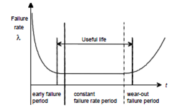
• The “Bx/Lx” metric is not limited to the classical reliability concept that reliability is only concern with failure that occur within the hypothetical useful service life (i.e. constant failure rate exponential distribution portion of the Bathtub Hazard Life curve).
• A “Bx/Lx” metric is inclusive of failures at all phases of the Bathtub curve which includes “Infant Mortality” (i.e. Quality issues) and “End of Life Wearout issues in addition to the “Random Failures” addressed by MTBF/MTTF metrics.
• This is the way the real world perceives Reliability as an accumulation of Infant Mortality Quality, Random Reliability and Durability Wearout (QRD) discrepancy and failure issues regardless of the origin of the problem.  (Note: The QRD philosophy for combining all product assurance disciplines started at General Motors in the late 1990 and continues to spread throughout the auto industry).
• Since “Bx/Lx” is so obvious and intuitive it is easily comprehended by non reliability personnel.  Therefore the frequent misuses and misunderstandings with MTBF/MTTF metric can be eliminated.
• Reliability professionals would no longer have to be endlessly trying to education the rest of the world on the probability theory and statistics math the limited arcane MTBF/MTTF metrics are based upon.

Figure 1: The Reliability Hazard Function Bathtub Curve

With respect to Dick Schmidt and his post on what I expect to be an enlightening paper that I hope to read some day, we have to consider if in today’s demanding, busy world, can we practically expect non-reliability managers, executives and colleagues to read and comprehend a 67 page thesis on mathematics for system reliability so they can understand “Our Reliability Speak”.  Especially when it was found to be too long for even the RIAC Reliability Journal that caters specifically to reliability professionals.

Or is it more practical for reliability professionals to
simply communicate in a language and use metrics
that are already widely understood by the rest of the world.

When I evolved from being an electronic design engineer and later an Electrical/Electronics (E/E) group manager to being the E/E reliability manager at an automotive OEM, I was involved in the elimination of MTBF/MTTF reliability requirements and all forms of actuarial reliability predictions such as MIL-HDBD-217 and all of its progeny back in the early 1990.  Back then the requirement for automotive E/E modules became a minimum of a 97% Reliability over 10 yrs of N. American Environmental Exposure and 100,000 Miles of Vehicle Usage that had to be demonstrated with a statistical confidence of at least 50%.  In other words a L3 (3.0% failure maximum) at 10 years AND 100K miles.  (Note: as a member of the SAE E/E reliability council I have seen that reliability requirements for automotive electronics have gotten more stringent since then.)

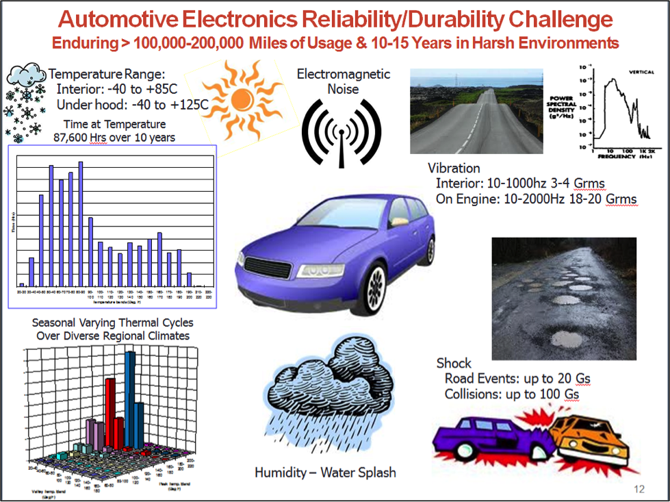
The vehicle life experience for the specific type of vehicle electronic module (i.e. Engine computer, Antilock Brake Module, Instrument Cluster, Radio . . . etc.) would then be defined in detail (See Figure 2). This would include:

• The hot & cold climatic extremes for N. American (or any other regions we were designing vehicles for) were defined in terms  of:
  • Time at Temperature,
  • Number and Type of Thermal Cycles,
  • Vibration and Shock
  • Humidity, Road Splash, Dust and Corrosive Road Salt Exposure
  • Etc.
• Usage profile were also defined in terms of
  • Ignition on and Engine Running Operating Hours,
  • Number of Power up /Power Down Operating Cycles,
  • Electrical Load Activation Cycles and Durations
  • Etc.

Figure 2: Environmental and Usage Conditions that Automotive Electronics Must Endure

This environmental and usage loading and stress information would be used to define and develop the accelerated reliability/durability demonstration test for the device or system where the confidence value was used to define the number of prototypes to be tested.  Our suppliers easily understood and implemented these requirements.

This “Bx/Lx” reliability requirement would then be used throughout the service life cycle of the vehicle.  The max allowable failure value would be prorated back against 120 months and fed into the companies warranty management computer system.  When dealership monthly warranty repair report came in, the number of service claims for each item in the vehicle would be compared against the life time reliability curve for the corresponding month of age.  For items where the number of actual service claims exceed the prorated limit line the warranty/service management computer issued a trip wire alarm bell alert for each item in violation of the failure/service event limit line.  A QRD issue resolution engineer would then be assigned to work with the part’s supplier to start a root cause investigation of why the part or system was exceeding the failure/service objective.

I led automotive E/E QRD improvement teams for about 3 yrs, sometime we would find a supply chain quality spill, or a design issue or the part was being misassembled or damaged at the vehicle assembly plants.  Other times we found the vehicle owner did not properly use the system or disliked how it worked, sometime we found the dealership misdiagnosed a problem and replaced the wrong part.  These latter issues were more prone to occur when a new technology system or feature was being introduced.

It never mattered if this was a Q, R or D issue.  We never said that is a quality department issue not a reliability issue.  The only thing that mattered was that there was some type of field problem that dissatisfied the end user customers and was costing us dealership repair time/dollars and might also cost us future vehicle sales.  Continuous QRD improvement was achieved by developing and implementing permanent corrective actions ranging from fixing quality spills to redesigns to improved training for assembly or repair technicians, were developed and implemented.

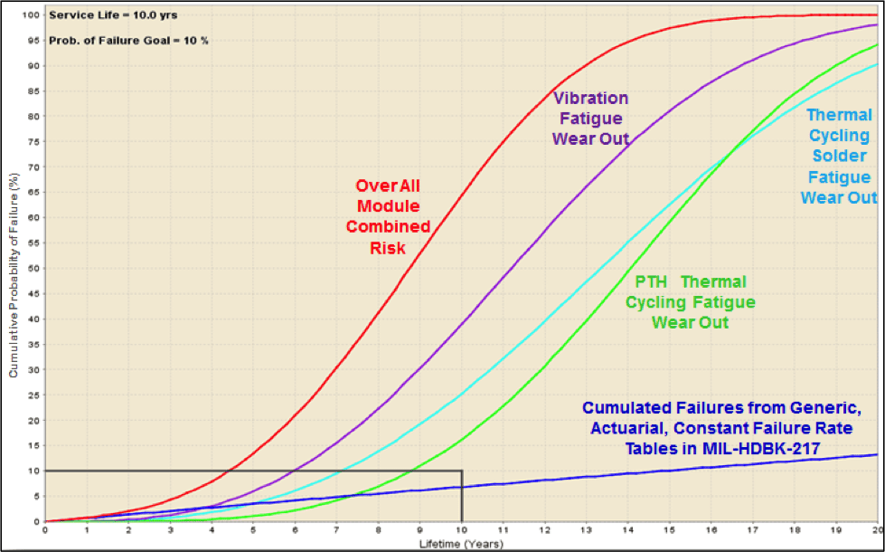
The “Bx/Lx” reliability metric is also seeing growing use in Physics of Failure (PoF) Durability Simulation based Reliability Assessments.  Figure 3 shows a plot of the individual and combined accumulated wearout failure risk timeline curves for an electronic module calculated from a Physics of Failure durability simulation produced using the Sherlock ADA PoF CAE App.  (Ref: http://www.dfrsolutions.com/software/the-future-of-design/).

(Ref: http://electronicdesign.com/automotive/physics-failure-durability-simulations-accelerate-development-and-improve-reliability-and).

10 Year L10 Reliability-Durability Objective  Figure 3: Physics of Failure Cumulative Failure Risk Life Curves for an Electronic Module

1. Produced by a Sherlock ADA PoF CAE App Durability Simulation.
   Overall Module & Individual Wearout Mechanism Failure Risks
   Compared to a Traditional MIL-HDBK-212 Reliability Prediction that Assumes a Constant MTBF
   Plotted against a 10 year L10 Reliability-Durability Objective.

This module has a 10 year L10 reliability-durability objective (i.e. no more than 10% failures (at least 90% Reliability) by 10 years in service.  The PoF analysis results plot reveal when each wearout failure mechanism is calculated to start and its related growth rate thereafter.  The near straight dark blue line at the bottom of the plot in Figure 6 shows the cumulated failures over time from a MIL-STD-217 rev F. part counting reliability prediction of the module that produces a constant failure rate (Inverse of MTBF) due to its limited focus on only the Random Failure portion of the Reliability Hazard function Bathtub curve.

The plot shows how traditional MTBF (i.e. Constant Random Failure Rate) reliability predictions can miss other reliability risks related to wearout issues when compared against a Reliability/durability objective.

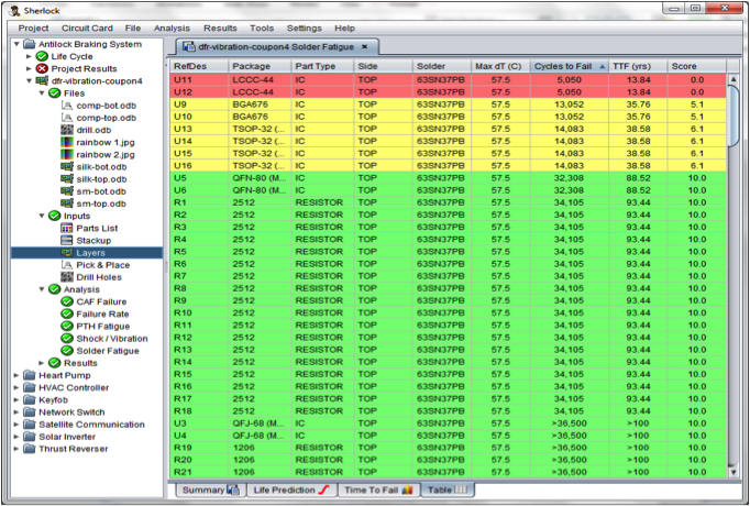
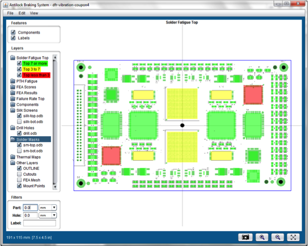
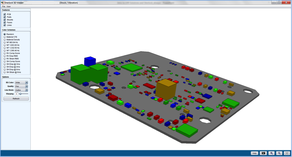
The PoF CAE App analysis also produces an ordered Pareto list that identifies the components or features projected to have the greatest risk of failure for each failure mechanisms.  The “Bx/Lx” reliability metric is again used by the CAE App program to assign Red – High Failure Risk, Yellow – Moderate Failure Risk and Green – No Failure Risk critically color coding to the Pareto list and the components sites in either 2D or 3D virtual models of the circuit board assembly as shown in Figure 4.  This enables easy identification and prioritization of all the weak link items, most likely to fail within the desired service life defined by the “Bx/Lx” Metric.  Correlation to failure risks to specific failure mechanism also identifies why they are expected to fail so that corrective actions can be implemented to design out the high risk items while the design is still on the CAD screen.  This virtual form of Reliability Growth can be achieved without the time and expense of building prototype modules and running physical reliability growth durability testing.

 

Figure 4: Pareto List and Color Coded 2D & 3D Graphic Representation of Component Failure Risks

SUMMARY:

This discussion illustrates that the “Bx/Lx” reliability metric which represents all QRD events across the entire service life can be used as an alternative to the MTBF/MTTF reliability metric which represent only random failures that occur during the hypothetical useful life portion of the product life cycle.

The “Bx/Lx” reliability metric already exists, is widely used in the bearing and machine industry, it predates MTBF/MTTF metrics and it can help foster continuously QRD growth throughout the product life cycle which includes development /qualification testing and evaluation of field reliability and failure repair rates.

The “Bx/Lx” metric is obvious, intuitive, and is easily comprehended by non-reliability professional in the real world.  Therefore the frequent problem related with non-reliability personnel not understanding or misusing the MTBF/MTTF metric can be eliminated.

I hope this paper inspires more discussion on how the reliability professions needs to think outside of the classically defense industry reliability box and think about the true big QRD picture in order to develop better reliability communication alternatives that solve the numerous problems with the MTBF/MTTF metrics.

About the Author: James G. McLeish, ASQ, SAE, IEEE

jmcleish@dfrsolutions.com 

James McLeish located in Rochester Hills Michigan heads the Mid-West Regional office of DfR Solutions a Failure Analysis/Lab Services Quality/Reliability/Durability (QRD) consulting and CAE APP Software Development firm.  He holds a MSEE degree, is a senior member of the ASQ Reliability Division, and a member of the SAE-Automotive Reliability Standards and ISO-26262 Functional Safety Committees.  He has over 35 years of automotive, military and industrial E/E design engineering and product assurance experience.  He started his career as an electronics product engineer who helped invent the first microprocessor based engine computer at Chrysler in the 1970’s.  He has since worked in systems engineering, design, development, product, validation, reliability and quality assurance of both E/E components and vehicle systems at General Motors and GM Military.  He holds 3 patents in embedded control systems, is an author or co-author of 3 GM E/E Validation Test / Reliability-Durability Demonstration standards.  He is credited with the introduction of Physics of Failure/Reliability Physics methods to GM while serving as a Reliability Manager and QRD Technical Expert.