
How to Do Residual Analysis to Check Your Statistical Models
The analysis of residuals helps to guide the analyst when analyzing data. It provides a way to select the model, analyze the data, develop parameter estimates, and to develop confidence in the results.
Linear Regression Model
During regression analysis, a model is selected. For example a linear equation may be assume to model a set of x-y data pairs. The parameters of the line that minimizes the sum of squares error are estimated. The residuals are the differences between the best-fit line and the actual data pairs. The linear model is
$$ \displaystyle\large \hat{y}_i=a+b*x_i $$
Here the y is a predicted value, a is a constant, b is the slope, and xi is a point on the line. The residuals are calculated as
$$ \displaystyle\large r_i=y_i-\hat{y}_i=y-a-b*x_i $$
The (xi, yi) pairs are the original data.
The residuals should follow a normal distribution and display only random patterns. Statistical methods, like the Kolmogorov-Smirnov test, can provide a numerical measure of normality. Assessing randomness require graphical methods where the residuals are plotted vs. another factor.
Linear Regression Example
We have set of 20 x-y data pairs where x is the independent variable and y is the dependent variable. We want to determine the best-fit line through the set. First create a scatter plot.
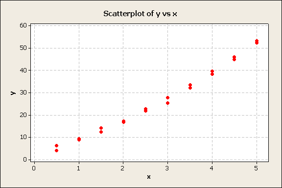
The scatter plot showed a strong linear trend so we decide to try a first order linear regression of y on x. This showed a good fit with a correlation of 98.6% and error standard deviation of 1.92. The parameter estimates for the intercept and the slope were statistically significant. Frequently, an analyst would stop here because of the high correlation. However, lets look the residuals using a probability plot.
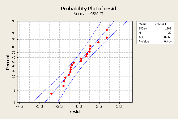
The bulk of the data follows a normal pattern, the blue line. Next, the residuals were plotted against x.
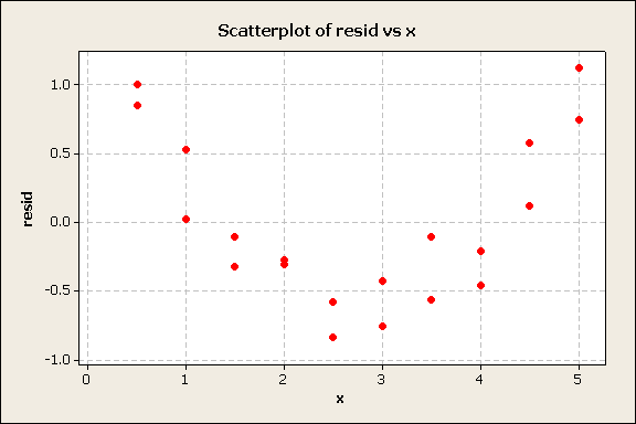
The curvature in the residuals plot suggests that there is a quadratic component that should be included in the analysis. The quadratic model is
$$ \displaystyle\large \hat{y}=a+b*x+c*x^2 $$
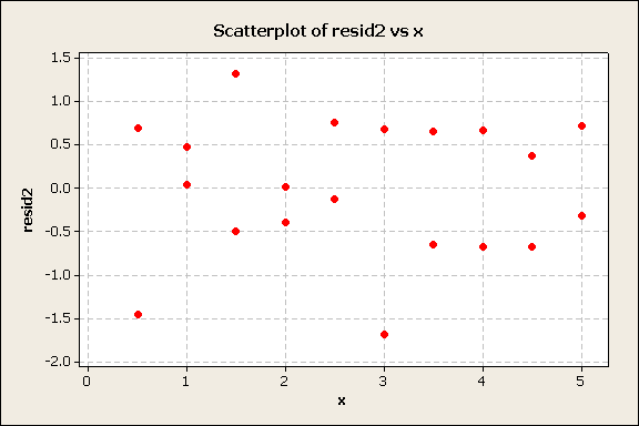
Using the quadratic model increased the correlation from 98.6% to 99.7% and reduced the error standard deviation from 1.92 to 0.83. The intercept, linear, and quadratic parameters were statistically significant. A plot of the residuals vs. the fitted values shows the expected randomness.
All of the above is mathematical statistics and easy to perform with statistical software. However, it is up to the user to judge it’s practical importance. In the engineering community, the first order linear regression may be sufficient. If one is in research, then the quadratic model may be important to a researcher may want to understand factors that cause the non-linearity. If projections are to be made outside of the range of data, then the quadratic model will probably provide better projections.
Design of Experiments Example
G.E.P. Box and D.R. Cox published a paper on toxins and treatments. In the study, animal survival times were recorded for four treatments of three poisons. A full factorial test design was use and four animal tests were conducted for each of the twelve treatment-poison combination. The DOE model is
$$ \displaystyle\large y_{i,j}=a+T_i+P_j $$
where i=1,2,3,4 and j=1,2,3
Here, the yij are the survival times, a is a constant, Ti are the four treatment, and Pj are the three poisons. The results of the analysis showed that treatments and poisons were all statistically significant, i.e., at least one treatment levels and at least one poison levels were statistically different. The error standard deviation was 0.16, and the correlation coefficient was 65%. This correlation is not very high.
The residuals were plotted against the predicted values.
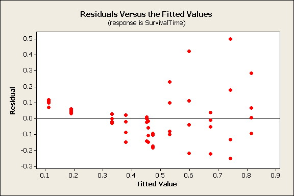
This plot shows the residuals have more variation on the right side of the graph than on the left side, a fan pattern. If the residuals were distributed randomly and followed the normal distribution, the spread would be more uniform across the plot.
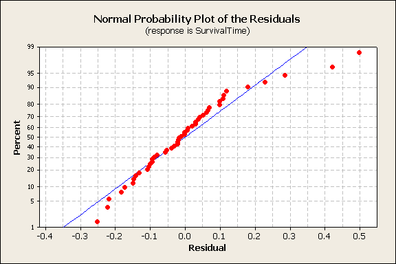
As another check, the normal probability plot of residuals shows some deviation from the ideal (blue) line and outliers at high residual values.
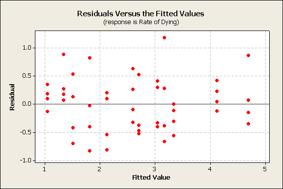
The analysis was repeated using a different response variable, i.e., the rate of dying 1/yij. Again, the treatment and poison factors were significant. Now a plot of the residuals vs. fitted values showed the expected random pattern.
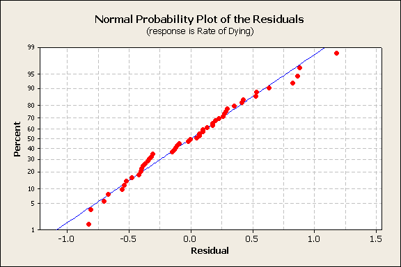
A normal probability plot of the residuals shows a normally distributed pattern.
From the analysis, it is clear that the best equation treatment x poison experimental result is
$$ \displaystyle\large 1/y_{i,j}=a+T_i+P_j $$
Conclusion
In the regression problem, the plot lead directed the analysis to assume a linear relationship between x and y. After analyzing the residuals, it was clear that a quadratic component would improve the model.
The DOE was a research study to build knowledge about poisons and treatments. Using residuals, the best response variable was found to be the rate of dying, not the survival time. This metric could be applied to future research.
That`s a great article that help bring us to think in the effects that we have when applying a model that hasn’t been tested or/and doesn’t have a good fit with the data set in study. Hence, applying GOF is proved a step that can’t be jumped when doing a reliability analysis.