Sample Sizes – Surveys
Introduction
How many responses are needed for a survey? This question requires specifying the desired confidence and the accuracy of the survey results.
The Bernoulli Trial
A Bernoulli trial is an event that has two possible outcomes. Consider the case where the only possible outcomes are success or failure. Let the probability of a success is p and the probability of failure equals q. The probabilities of all possible events must equal 1, so q = 1-p. These relationships are expressed mathematically as
$$Pr(Success)=p$$
(1)
$$Pr(Failure)=q=1-p$$
(2)
Examples of a Bernoulli trial would be a survey where a participant must indicate their sex as male or female, manufactured parts that conform or fail inspection, or perhaps the roll of a dice produces a 6 or not a 6.
In an unbiased survey, the number of males and females should be about equal, so p is approximately 0.5. In a mature manufacturing operation, the probability of a failed part should be very low or 0. With a fair dice having 6 unique faces, the probability of obtaining a 6 is p=1/6. In these examples, all outcomes have been considered, so the probability p ranges from 0 to 1.
Binomial
We estimate the probability p by using a group of n Bernoulli trials which yield x successes and n-x failures. The value of p is estimated by
$$p=\frac{x}{n}$$
(3)
The value of p from an unbiased statistical sample should be close to the population value of p. However, different samples of size n will have different values for x. This means x and the calculated p value are random variables.
The x values are binomially distributed. The probabilities are provided by the Binomial Equation
$$Pr(x)=\lgroup{\frac{x}{n}}\rgroup p^x(1-p)^{n-x}$$
(4)
Where the number of combinations, order unimportant, of successes and failures, is
$$\lgroup{\frac{x}{n}}\rgroup = \frac{n!}{x!(n-x)!}$$
(5)
And the factorial of integer N is defined as
$$N!=N(N-1)(N-2)…(2)(1)$$
(6)
It can also be shown that the probability of all possible events equals 1
$$1=\sum_{x=0}^{x=N}{\lgroup{\frac{n}{x}}\rgroup p^x(1-p)^{n-x}}$$
(7)
Mean and standard deviation of the Binomial distribution, equation 4, are
$$\mu_p=p$$
(8)
And
$$\sigma_p^2=\frac{p(1-p)}{N}$$
(9)
Simulation
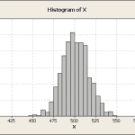
Minitab was used show to create a simulation of the Binomial distribution. A simulation of 1000 Bernoulli trials was made and the number of successes (X) were counted. The results were plotted as a histogram, figure 1.
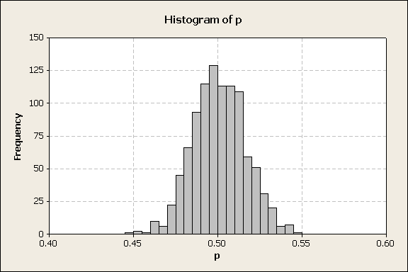
Figure 1
This shows that while the surveys follow a binomial distribution, the distribution of surveys can be approximated by a normal distribution, assuming large survey sample sizes. From the simulation, the $-\bar{x}=500.42-$, $-s_x=15.68-$, and the $-6s=94.08-$.
Now divide the X’s by N to obtain a histogram of the p values, figure 2.
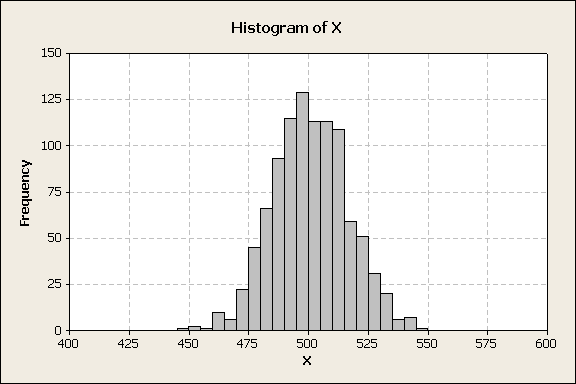
Figure 2
From the simulation, $-\bar{x}=0.50042-$ and $-s_p=0.01568-$. Again, p, µ, and σ population values are all unknown parameters, but are estimated from simulation data.
The normal approximation works best when p is close to 0.5 and when the sample size is large. A more precise criteria is to apply the normal approximation when np>5 and n(1-p)>5. (Some references specify np>10 and n(1-p)>10). If p=0.5, then the normal approximation works when n>10. If p=0.1 (or p=0.9) then n>50. Similarly, if p=0.01, then n>500.
Confidence
Our confidence in the survey results increases with sample size. However, it is desirable to have an objective way to determine the sample size required to develop a specified confidence. Generally surveys use very large sample sizes so the normal approximation is justified. Using the normal approximation, the µ and σ survey results are used to calculate a two-sided confidence interval with equation
$$\mu+z_{\alpha/2}\sigma<p<\mu+z_{1-\alpha/2}\sigma$$
(10)
Here, $-\alpha-$ is the percent of the population that lies in the tails of the distribution, z is the number of standard deviations, $-z_{\alpha/2}-$ is the z value for the lower tail, and $-z_{1-\alpha/2}-$ is the z value for the upper tail. This confidence interval contains $-C=1-\alpha-$ of the distribution.
If we desire 90% confidence limits, then α=0.10. Then z0.05 = -1.96 and z0.95 = 1.96. The 90% confidence interval width is . Then the 90% confidence interval width is
$$\Delta=2(1.96)\sigma_p=3.92\sqrt{\frac{p(1-p)}{N}}$$
(11)
To calculate the sample size N that supports a specified precision at 90% confidence use
$$N=\frac{15.37}{\Delta^2}p(1-p)$$
(12)
Example 1
Two political candidates are in a close election. The approximate p value is 0.5 for both candidates. We would like to know a candidate’s probability of success with a 90% confidence interval of $-\pm1%-$. Then the minimum number of survey responses is
$$N = \frac{15.37}{0.02^2}(0.5)(1-0.5)=9,606$$
(13)
A reasonable plan would be to obtain 10,000 survey responses. However, surveys have a history of low response rates. If the number of survey responses is less, then confidence would be reduced or the confidence interval width increased.
Example 2
Consider a situation where there are 4 candidates competing for a political party’s nomination. We want to consider a candidate’s chance vs. the rest of the candidates. Success is the candidate being selected. Failure is an alternate candidate being selected in the Bernoulli trials. Assuming an equal chances, then each candidate has a success probability of $-p=0.25-$. The failure probability is $-q=1-p=0.75-$. The minimum survey size required for a confidence of $-\pm1%-$ is
$$N=\frac{15.37}{0.02^2}(0.25)(1-0.25)=28,819$$
(14)
A reasonable sampling plan would target 29,000 responses to know p within $-\pm1%-%, the candidate’s chances of winning the nomination.
General Sample Size Equation
Different individuals or organizations require different confidence levels. The calculation may be generalized to C confidence. Since $-C=1-\alpha-$, then the upper tail $-z_{(1-C)/2}-$ yields
$$N=\frac{(2z_{(1-C)/2})^2}{\Delta^2}p(1-p)$$
(14)
Conclusions
- While individual survey responses follow a Bernoulli process, a group of surveys follows a Binomial distribution.
- At large sample sizes, the Binomial approaches a Normal distribution.
- The Normal distribution is used to determine the relationship between confidence limits, sample size, and p value.
- Surveys require a large number of responses to provide results that are precise and support desired confidence levels.
- Equation 14 provides a general equation to calculate the required survey sample responses.
Dennis Craggs, Consultant
810-964-1529
dlcraggs@me.com
I can be engaged on this or other topics. The first contact hour is free to discuss your problem/concerns and to determine how I can help you.
I have worked in Quality, Reliability, Applied Statistics, and Data Analytics over 30 years in design engineering and manufacturing. I teach at the Master’s level in graduate school, provide Minitab seminars to corporate clients, write articles, and have presented and written papers at SAE, ISSAT, and ASQ. I want to assist you.
Leave a Reply